
Appendix A: Conversion of Expressions from SI to FPS Units
This appendix provides the FPS equivalents of selected empirical expressions and equations presented in SI units in Part 6 of the Code. It may be noted that the computed values obtained from an SI expression and its FPS equivalent given in this Appendix may show some differences, which may be due to rounding off of the constants within these expressions. However, these differences, if any, may be only minor, and the FPS equivalent expressions are intended to serve as references only.Chapter 2
The following units are applicable to the corresponding variables in the expressions provided below.Chapter 4
The following units are applicable to the corresponding variables in the expressions provided below.Chapter 5
The following units are applicable to the corresponding variables in the expressions provided below.Chapter 6
The following units are applicable to the corresponding variables in the expressions provided below.Chapter 7
The following units are applicable to the corresponding variables in the expressions provided below.Chapter 8
The following units are applicable to the corresponding variables in the expressions provided below.Chapter 9
The following units are applicable to the corresponding variables in the expressions provided below.Chapter 10
The following units are applicable to the corresponding variables in the expressions provided below.Chapter 10 (Steel Structures) is by far the densest section of Appendix A, with well over a hundred paired expressions. Each row below reproduces one SI expression from the Code and its FPS equivalent, in the same order as the source table, grouped by the Section/Table reference given in the source (a blank Section/Table cell means the expression continues under the row above it).
Chapter 11
In the following equations, the unit of is mm in SI unit and inch (in) in FPS unit.Appendix B: Methods of Soil Exploration and Sampling
B1 Methods of soil exploration
The detailed methods of soil investigation usually includes collecting undisturbed samples and or performing field tests. Listed below are some of the common methods of subsoil exploration. a) Open trial pits: In this method trial pits are excavated exposing the subsoil thoroughly. Undisturbed samples are taken from intact sides and bottom of the trial pits. This is suitable for all types of formation but for cuts which cannot stand below water table, proper bracing shall be provided. This method is normally used for shallow depths (up to 3 m). b) Auger boring: Augers, hand or power operated, are rotated and forced into soil. Augers are withdrawn and emptied when full. Soil cuttings obtained are used to interpret stratification and soil type. The method is unsatisfactory for cohesionless soils above or below ground water. c) Shell and auger boring: Manual or mechanized rigs are used for vertical boring. The tools consist of auger for soft to stiff clays, shells for very stiff to hard clays, shells or sand pumps attached to sectional boring rods for sandy strata. d) Wash boring: In this method, soil is loosened by chopping and cutting by impact and twisting action of a lightweight bit. Soil is removed from the borehole by a stream of water or drilling mud from lower end of the wash pipe which is worked up and down or rotated into the borehole. The water or mud flow carries the soil through the annular space between the wash pipe and casing and is overflown at ground level. The soil in suspension is allowed to settle in a pond or tank and the fluid is recirculated as required. The soil brought to surface by the wash water can be used for identification purposes but is not representative of the character and consistency of the material penetrated and the flushing water may disturb the surrounding ground. Subsoil can be identified throughly if field tests (viz. Standard Penetration Test) are performed and or undisturbed samples are collected frequently. e) Sounding/probing: A number of sounding methods are available. The most common is the Standard Penetration Test (SPT)1. The SPT test is specified both in reference 1 and in ASTM D1586. Other methods include procedures like Cone Penetration Test (CPT)2 and Dynamic Probing (DP)3. Sounding/probing may be done in conjunction with inhole tests such as “Field Vane Shear Test in Cohesive Soil”, (ASTM D2573), bore-hole shear (Iowa Bore-hole Shear) Test, Flat Dilatometer Test (DMT)4 or “Pressuremeter Tests in Soils”, (ASTM D4719).Numerals in the superscript in this paragraph refer to the corresponding reference materials cited in the list of references in Sec B4 in this appendix.
B2 Choice of method
The choice of a method of soil exploration depends upon: a) the topography, type of ground to be investigated and ground water conditions; b) the type of building envisaged and technical requirements; c) amount of existing information; d) expected variability of soil; e) external constraints such as availability of plant, access, cost and time. The technical requirements of the investigation rather than cost should be the overriding factor in the selection of exploration method. In clayey soils, borings are suitable for deep exploration and pit for shallow exploration. In sandy soils special equipments are needed for taking representative samples below the water table. Ground investigation is normally done by boreholes, but where only shallow depths are to be investigated, and where ground water problems are not envisaged, trial pits may prove more versatile and economical. Boreholes may be necessary on waterlogged sites where it is impracticable to excavate trial pits without dewatering. Safety aspects must be considered when selecting and carrying out exploration. Precautions relating to safety, health and welfare of workmen, hazards from underground services, contaminated ground and inspection pits or shafts shall be undertaken. Overhead power lines are a hazard if ground investigation rigs are to operate in the vicinity.B3 Sampling methods
Sample quality is dependent on type of soil being sampled, type and condition of equipment and the skill with which it is used. The weaker material is the most significant in an investigation, and is usually difficult to secure in an undisturbed condition. It is rarely possible to sample granular (non-cohesive) materials in undisturbed condition, unless special techniques are used. Granular soil conditions are usually assessed by in-situ tests and confirmed by disturbed samples which permit classification and grading analysis and visual inspection. Cohesive soils may be tested both in-situ and in laboratory on undisturbed or relatively undisturbed samples. Based on assessment of the quality, samples can be classed into five categories as specified in Table B1. Table B1: Categories of Soil Samples Based on Quality
The sample and/or test locations must be such that all changes of stratum are recorded. A number of extra samples and test results are usually required to assess variation of the properties of a stratum with depth. The record of all borings shall include the following information:
a) Size of casing (if used),
b) Number of blows per 300 mm required to drive the sampling spoon,
c) The elevation of the ground surface referred to an established datum,
d) Location and depth of boring and its relation to the proposed construction,
e) Elevation at which samples were taken,
f) Elevation of the boundaries of soil strata,
g) Description of the soil strata encountered and any particular unusual or special condition such as loss of water in the earth and rock strata, presence of boulders, cavities and obstructions, use of special type of samplers, traps, etc., and,
h) The level of ground water together with a description of how and when it was observed.
All abandoned and unsuccessful attempts of borings or drillings shall also be reported. In complex formations, details of sampling are necessary and, therefore, separate holes may be employed purely for sampling or testing, termed as double hole sampling.
Care shall be taken in protecting, handling, labelling and subsequently transporting the samples, so that samples can be received in a fit state for examination and testing, and can be correctly recognized as coming from a specific trial pit or boring.
Class 1 and Class 2 samples listed in Table B1 are generally referred to as ‘undisturbed’ while Classes 3, 4, and 5 as ‘disturbed’ samples.
a) Disturbed samples: These are taken by methods which modify or destroy the natural structure of the material though with suitable precaution the natural moisture content can be preserved. The amount of sample generally required for testing purposes is given in Table B2.
b) Undisturbed samples: These are taken by methods which preserve the structure and properties of the material. Truely undisturbed samples can not be taken from boreholes, and in practice there are only differing levels of disturbed samples. Material may be secured in open tube samplers for clays except of firm or of stiff consistency. For softer clays stationary piston samplers of low area ratio*, shall be used and careful boring and sample preservation technique shall be employed. The minimum diameter of undisturbed sample shall be 40 mm with minimum length/diameter ratio of 3.
* The area ratio is defined as the ratio of the volume of soil displacement to the volume of the collected sample, expressed as a percentage;
where
= outside diameter of tube
= inside diameter of cutting edge.
Well designed sample tubes should have an area ratio of less than about 10 per cent.
c) Representative samples: These samples have all their constituent parts preserved, but may or may not be structurally disturbed.
Table B2: Weight of Soil Sample Required for Laboratory Tests
B4 List of references
- ISSMFE, TC-16, Report of the Technical Committee on Penetration Testing of Soils, International Reference Test Procedures for Standard Penetration Test; Swedish Geotechnical Society; Swedish Geotechnical Institute, Appendix B: ISSN 0281-7578 (1989)
- ISSMFE, TC-16, Report of the Technical Committee on Penetration Testing of Soils, International Reference Test procedures for Cone Penetration Test (CPT): Swedish Geotechnical Society; Swedish Geotechnical Institute, Appendix A: ISSN 0281-7578 (1989)
- ISSMFE, TC-16, Report of the Technical Committee on Penetration Testing of Soils, International Reference Test Procedures for Dynamic Probing (DP): Swedish Geotechnical Society; Swedish Geotechnical Institute, Appendix C: ISSN 0281-7578 (1989)
- Merchetti, S. “In Situ Tests by Flat Dilatometer”, Journal, GTE Divn., ASCE, Vol 106, GT 3, March, pp. 299-321 (1980).
Appendix C: Guidelines for Computing the Column Interaction Diagrams
C1 General
The interaction diagram of a given column section is drawn by assuming a series of strain distributions, each corresponding to a particular point on the interaction diagram, and computing the corresponding values of axial load and moment . Once enough such points have been computed, the results are summarized on an interaction diagram. In this appendix, the method and relationships needed to compute the various points on an interaction diagram are given based on strain compatibility and mechanics. The calculations involve the assumptions stated in Sec 6.2.3.1 through 6.2.3.7 and Sec 6.3.3.2 of Part 6.C2 Computation of interaction diagram
The various controlling points of an interaction diagram are shown in Fig C1.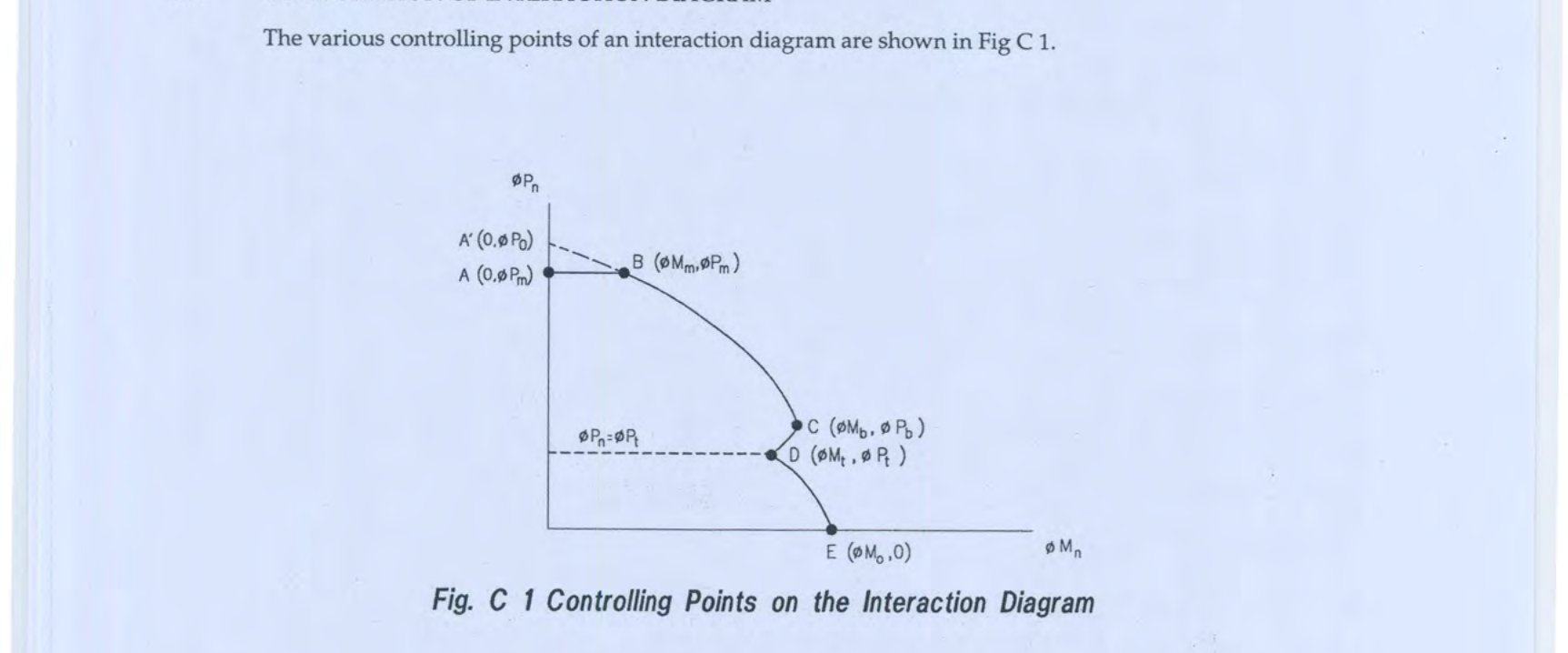
C2.1 Computation of Point A
The maximum usable axial load is represented by point A on the interaction diagram. The maximum axial load shall be calculated as where is given by Eq (6.3.1) for spiral columns and by Eq (6.3.2) for tied columns. Once is evaluated, a horizontal straight line shall be drawn through A. This line shall mark the upper boundary of the interaction diagram.C2.2 General Case
Point A’ in Fig C1 represents the theoretical maximum (but not usable) axial load for a column under truly concentric loading. This theoretical maximum axial load is calculated as For a symmetrical section, the corresponding moment will be zero. For unsymmetrical columns, provided the moments are taken about the geometric centroid of the section, Eq (C 10) may be used to compute the moment corresponding to . Point E on the interaction diagram can be obtained by evaluating the moment capacity, , for pure flexure with no axial load. While point A’ is outside the interaction diagram and the portion of curve between A’ and B is not usable, the solution of the general case applies for the entire curve A’BCDE. For the purpose of this general solution, the longitudinal column bars will be considered in layers perpendicular to the plane of bending. Layer 1 is closest to the “least compressed” surface and is at a distance from the “most compressed” surface. Layers 2, 3, 4 etc. are successively away from the least compressed surface and at distances etc. respectively from the most compressed surface. Each strain distribution to be considered is linear with the maximum compressive strain in concrete . Layer 1 will have a strain and area , layer 2 strain and area and so on. The strain distribution will be defined by setting and , where is the strain in steel at the onset of yield. Each strain distribution considered will correspond to a different arbitrarily chosen strain ratio , where positive values of correspond to positive (compressive) strains. For example, corresponds to , the yield strain in tension. If and are the strain in the th layer of steel and the depth to that layer from the most compressed surface respectively, where is the depth of the compression zone given by Once the values of and and so on, are known, the stress in each layer of steel is computed as The concrete stress is uniform over the equivalent rectangular stress block having a depth where is given in Sec 6.2.3.7(c). The compressive force in concrete is given by where is the area of the compression zone. For a rectangular section, , in which is the width of the section. For a nonrectangular section, is the area of the compression zone having a depth , measured perpendicular to the neutral axis. If is less than for a particular layer of steel, the force in that layer of steel is given by If is greater than for a particular layer of steel, the force in that layer of steel is The axial load capacity, for the assumed strain distribution is obtained as The corresponding moment capacity, for an assumed strain distribution, taken about the centroid is given by where is the overall dimension of the concrete cross-section parallel to the plane of bending, and is the distance of the centroid of compression zone from the centroid of the section.C2.3 Computation of Point C
Point C on the interaction diagram of Fig C1 corresponds to the balanced condition ( in tension) and is obtained from Eq (C 3) through (C 10) using . Once and are evaluated from Eq (C 9) and (C 10), point C can be located as in which the values shall be taken as follows: for tied columns, and for spiral columns.C2.4 Determination of Portion BC
Portion BC of the interaction diagram can be constructed by repeated application of Eq (C 3) through (C 10) for various values of the strain ratio . The recommended sequence of strain ratios are and . Of these, points corresponding to (zero tension in steel), (maximum steel tension 25% of ), (maximum steel tension 50% of ) and (maximum steel tension ) should always be determined. The points on the curve are for each value of , where is to be taken as 0.7 for tied columns, and 0.75 for spiral columns. Once adequate points are plotted, portion A’C can be drawn. The intersection of this curve with the horizontal line through A locates point B.C2.5 Determination of Portion CD
Portion CD of the interaction diagram of Fig C1 can be obtained by taking negative values of beyond , such as and so on, and using Eq (C 3) through (C 10). Each time the value of is to be taken as for tied columns, and for spiral columns. Once adequate points are plotted, the portion of curve CD (or its extension) should be drawn. The intersection of this curve with the horizontal straight line corresponding to locates the transition point D. Here, is the axial load capacity at the transition point D as given in Sec 6.3.5.C2.6 Determination of Portion DE
Once the transition point D is located, portion DE can be drawn by using Eq (C 3) through (C 10) for negative values of beyond . For this portion, however, an increased value of is to be used, as given in Sec 6.3.5, for the evaluation of and . Once the portion of curve DE (or its extension) is drawn, its intersection with the abscissa () locates point E.C3 Interaction diagram for circular columns
Equations (C 3) through (C 10) can also be used to determine the interaction diagram of a circular column. However, this time the compression zone is a segment of a circle, of depth , as shown in Fig C2. To compute the compressive force in concrete and its moment about the centroid of the section using Eq (C 6) and (C 10), the following parameters may be helpful. Area of the compression zone segment Distance of centroid of the compression zone segment form the centroid of the circular section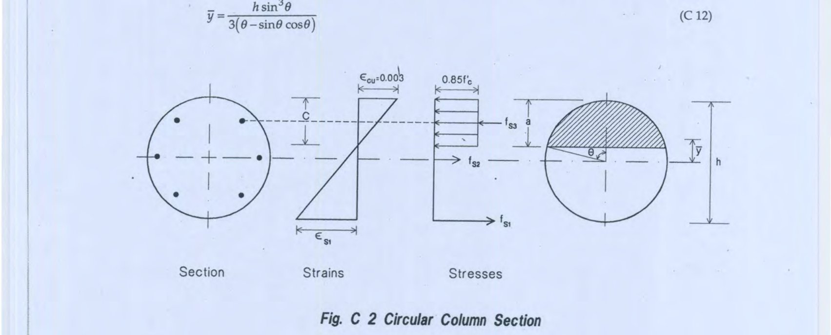
C4 Unsymmetrical section
For unsymmetrical sections, with different amount of steel on opposite sides of the neutral axis, the same procedure using Eq (C 3) through (C 10) can be employed for determining the interaction diagram. However, the balanced load for positive moment will be different from that for negative moment. In a similar manner, the maximum axial load capacity, corresponding to a uniform compressive strain of 0.003 across the section, will be accompanied by a moment.C5 Nondimensional interaction diagrams
It may be useful to express interaction diagrams independently of column dimensions. This can be done by dividing by and by and drawing the curves with as abscissa and as ordinate. A family of such interaction diagrams for various combinations of and with different reinforcement amounts and arrangements can be prepared to serve as design aids.Appendix D: Calculation of Volume Fraction of Reinforcement
The volume fraction of reinforcement in a ferrocement section can be readily calculated if the density of the mesh material and the weight of mesh per unit area are known. For ferrocement section reinforced with expanded metal mesh, the volume fraction of mesh reinforcement may be calculated from the following relationship. where,- = number of mesh layers
- = thickness of ferrocement section, mm
- = weight of mesh per unit area, N/mm²
- = unit weight of steel, N/mm³
- = number of layers of mesh reinforcement
- = diameter of mesh wire
- = thickness of ferrocement
- = centre to centre spacing of wires aligned transverseley in reinforcing mesh, mm
- = centre to centre spacing of wires aligned longitudinally in reinforcing mesh, mm
Appendix E: Common Types and Sizes of Steel Meshes used in Ferrocement
Table: Common Types and Sizes of Steel Meshes used in Ferrocement
* American wire gauge.
The source table’s “Expanded metal mesh” row packs the mesh-size designation (“18 N/m²”), the two gauge callouts, and their corresponding thicknesses (0.58, 1.00, 0.76 mm) into fewer columns than the wire-mesh rows above it — the mesh has no discrete wire spacing or AWG-numbered wire gauge in the same sense as woven/welded wire mesh. The values above are transcribed in the same left-to-right order as the source table.